Waveform

class ketos.audio.waveform.Waveform(data, time_res=None, filename='', offset=0, label=None, annot=None, transforms=None, transform_log=None, **kwargs)

Audio signal

Args:

rate: float

Sampling rate in Hz

data: numpy array

Audio data

filename: str

Filename of the original audio file, if available (optional)

offset: float

Position within the original audio file, in seconds measured from the start of the file. Defaults to 0 if not specified.

label: int

Spectrogram label. Optional

annot: AnnotationHandler

AnnotationHandler object. Optional

transforms: list(dict)

List of dictionaries, where each dictionary specifies the name of a transformation to be applied to this instance. For example, {“name”:”normalize”, “mean”:0.5, “std”:1.0}

transform_log: list(dict)

List of transforms that have been applied to this instance

Attributes:

rate: float

Sampling rate in Hz

data: 1numpy array

Audio data

time_ax: LinearAxis

Axis object for the time dimension

filename: str

Filename of the original audio file, if available (optional)

offset: float

Position within the original audio file, in seconds measured from the start of the file. Defaults to 0 if not specified.

label: int

Spectrogram label.

annot: AnnotationHandler

AnnotationHandler object.

transform_log: list(dict)

List of transforms that have been applied to this instance

Methods

add(signal[, offset, scale])	Add the amplitudes of the two audio signals.
add_gaussian_noise(sigma)	Add Gaussian noise to the signal
append(signal[, n_smooth])	Append another audio signal to the present instance.
bandpass_filter([freq_min, freq_max, N])	Apply a lowpass, highpass, or bandpass filter to the signal.
cosine(rate, frequency[, duration, height, ...])	Audio signal with the shape of a cosine function
from_wav(path[, channel, rate, offset, ...])	Load audio data from one or several audio files.
gaussian_noise(rate, sigma, samples[, filename])	Generate Gaussian noise signal
get_repres_attrs()	Get audio representation attributes
morlet(rate, frequency, width[, samples, ...])	Audio signal with the shape of the Morlet wavelet
plot([show_annot, figsize, label_in_title, ...])	Plot the data with proper axes ranges and labels.
resample(new_rate[, resample_method])	Resample the acoustic signal with an arbitrary sampling rate.
to_wav(path[, auto_loudness])	Save audio signal to wave file

add(signal, offset=0, scale=1)

Add the amplitudes of the two audio signals.

The audio signals must have the same sampling rates. The summed signal always has the same length as the present instance. If the audio signals have different lengths and/or a non-zero delay is selected, only the overlap region will be affected by the operation. If the overlap region is empty, the original signal is unchanged.

Args:

signal: Waveform

Audio signal to be added

offset: float

Shift the audio signal by this many seconds

scale: float

Scaling factor applied to signal that is added

Example:

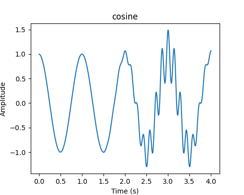
>>> from ketos.audio.waveform import Waveform
>>> # create a cosine wave
>>> cos = Waveform.cosine(rate=100, frequency=1., duration=4)
>>> # create a morlet wavelet
>>> mor = Waveform.morlet(rate=100, frequency=7., width=0.5)
>>> mor.duration()
3.0
>>> # add the morlet wavelet on top of the cosine, with a shift of 1.5 sec and a scaling factor of 0.5
>>> cos.add(signal=mor, offset=1.5, scale=0.5)
>>> # show the wave form
>>> fig = cos.plot()
>>> fig.savefig("ketos/tests/assets/tmp/morlet_cosine_added.png")
>>> plt.close(fig)

add_gaussian_noise(sigma)

Add Gaussian noise to the signal

Args:

sigma: float

Standard deviation of the gaussian noise

Example:

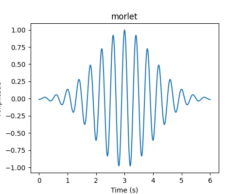
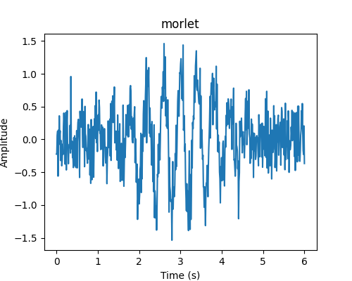
>>> from ketos.audio.waveform import Waveform
>>> # create a morlet wavelet
>>> morlet = Waveform.morlet(rate=100, frequency=2.5, width=1)
>>> morlet_pure = morlet.deepcopy() # make a copy
>>> # add some noise
>>> morlet.add_gaussian_noise(sigma=0.3)
>>> # show the wave form
>>> fig = morlet_pure.plot()
>>> fig.savefig("ketos/tests/assets/tmp/morlet_wo_noise.png")
>>> fig = morlet.plot()
>>> fig.savefig("ketos/tests/assets/tmp/morlet_w_noise.png")
>>> plt.close(fig)

append(signal, n_smooth=0)

Append another audio signal to the present instance.

The two audio signals must have the same samling rate.

If n_smooth > 0, a smooth transition is made between the two signals by padding the signals with their reflections to form an overlap region of length n_smooth in which a linear transition is made using the _smoothclamp function. This is done in manner that ensure that the duration of the output signal is exactly the sum of the durations of the two input signals.

Note that the current implementation of the smoothing procedure is quite slow, so it is advisable to use small value for n_smooth.

Args:

signal: Waveform

Audio signal to be appended.

n_smooth: int

Width of the smoothing/overlap region (number of samples).

Returns:

None

Example:

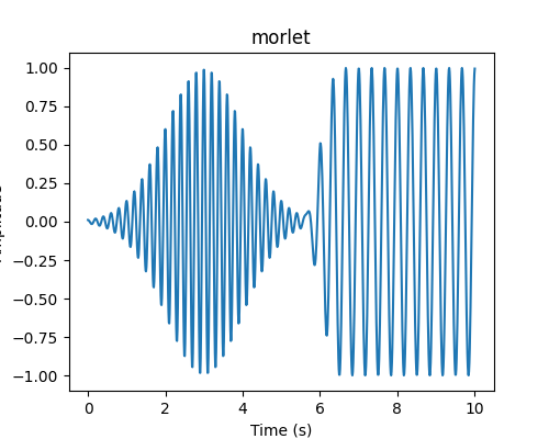
>>> from ketos.audio.waveform import Waveform
>>> # create a morlet wavelet
>>> mor = Waveform.morlet(rate=100, frequency=5, width=1)
>>> # create a cosine wave
>>> cos = Waveform.cosine(rate=100, frequency=3, duration=4)
>>> # append the cosine wave to the morlet wavelet, using a overlap of 100 bins
>>> mor.append(signal=cos, n_smooth=100)
>>> # show the wave form
>>> fig = mor.plot()
>>> fig.savefig("ketos/tests/assets/tmp/morlet_cosine.png")
>>> plt.close(fig)

bandpass_filter(freq_min=None, freq_max=None, N=3)

Apply a lowpass, highpass, or bandpass filter to the signal.

Uses SciPy’s implementation of an Nth-order digital Butterworth filter.

The critical frequencies, freq_min and freq_max, correspond to the points at which the gain drops to 1/sqrt(2) that of the passband (the “-3 dB point”).

Args:

freq_min: float

Lower limit of the frequency window in Hz. (Also sometimes referred to as the highpass frequency). If None, a lowpass filter is applied.

freq_max: float

Upper limit of the frequency window in Hz. (Also sometimes referred to as the lowpass frequency) If None, a highpass filter is applied.

N: int

The order of the filter. The default value is 3.

Example:

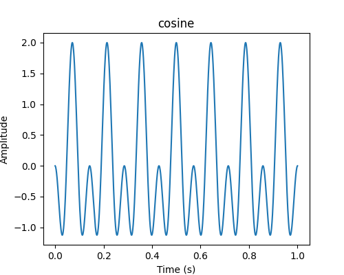
>>> from ketos.audio.waveform import Waveform
>>> # create a Cosine waves with frequencies of 7 and 14 Hz
>>> cos = Waveform.cosine(rate=1000., frequency=7.)
>>> cos14 = Waveform.cosine(rate=1000., frequency=14.)
>>> cos.add(cos14)
>>> # show combined signal
>>> fig = cos.plot()
>>> fig.savefig("ketos/tests/assets/tmp/cosine_double_audio.png")
>>> plt.close(fig)
>>> # apply 10 Hz highpass filter
>>> cos.bandpass_filter(freq_max=10)
>>> # show filtered signal
>>> fig = cos.plot()
>>> fig.savefig("ketos/tests/assets/tmp/cosine_double_hp_audio.png")
>>> plt.close(fig)

classmethod cosine(rate, frequency, duration=1, height=1, displacement=0, filename='cosine')

Audio signal with the shape of a cosine function

Args:

rate: float

Sampling rate in Hz

frequency: float

Frequency of the Morlet wavelet in Hz

duration: float

Duration of the signal in seconds

height: float

Peak value of the audio signal

displacement: float

Phase offset in fractions of 2*pi

filename: str

Meta-data string (optional)

Returns:

Instance of Waveform

Audio signal sampling of the cosine function

Examples:

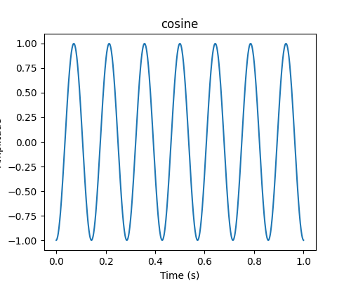
>>> from ketos.audio.waveform import Waveform
>>> # create a Cosine wave with frequency of 7 Hz
>>> cos = Waveform.cosine(rate=1000., frequency=7.)
>>> # show signal
>>> fig = cos.plot()
>>> fig.savefig("ketos/tests/assets/tmp/cosine_audio.png")
>>> plt.close(fig)

classmethod from_wav(path, channel=0, rate=None, offset=0, duration=None, resample_method='scipy', id=None, normalize_wav=False, transforms=None, pad_mode='reflect', smooth=0.01, **kwargs)

Load audio data from one or several audio files.

When loading from several audio files, the waveforms are stitched together in the order in which they are provided using the append method. Note that only the name and offset of the first file are stored in the filename and offset attributes.

Note that - despite the misleading name - this method can load other audio formats than WAV. In particular, it also handles FLAC quite well.

TODO: Rename this function and document in greater detail which formats are supported.

Args:

path: str or list(str)

Path to input wave file(s).

channel: int

In the case of stereo recordings, this argument is used to specify which channel to read from. Default is 0.

rate: float

Desired sampling rate in Hz. If None, the original sampling rate will be used

offset: float or list(float)

Position within the original audio file, in seconds measured from the start of the file. Defaults to 0 if not specified.

duration: float or list(float)

Length in seconds.

resample_method: str

Resampling method. Only relevant if rate is specified. Options are

• kaiser_best

• kaiser_fast

• scipy (default)

• polyphase

See https://librosa.github.io/librosa/generated/librosa.core.resample.html for details on the individual methods.

id: str

Unique identifier (optional). If provided, it is stored in the filename class attribute instead of the filename. A common use of the id argument is to specify a full or relative path to the file, including one or several directory levels.

normalize_wav: bool

Normalize the waveform to have a mean of zero (mean=0) and a standard deviation of unity (std=1). Default is False.

transforms: list(dict)

List of dictionaries, where each dictionary specifies the name of a transformation to be applied to this instance. For example, {“name”:”normalize”, “mean”:0.5, “std”:1.0}

smooth: float

Width in seconds of the smoothing region used for stitching together audio files.

pad_mode: str

Padding mode. Select between ‘reflect’ (default) and ‘zero’.

Returns:

Instance of Waveform

Audio signal

Example:

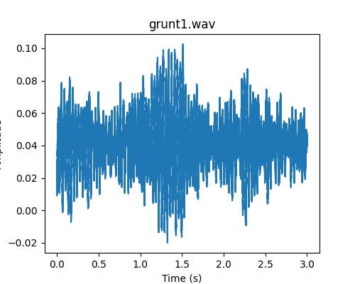
>>> from ketos.audio.waveform import Waveform
>>> # read audio signal from wav file
>>> a = Waveform.from_wav('ketos/tests/assets/grunt1.wav')
>>> # show signal
>>> fig = a.plot()
>>> fig.savefig("ketos/tests/assets/tmp/audio_grunt1.png")
>>> plt.close(fig)

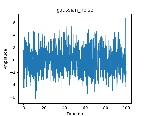
classmethod gaussian_noise(rate, sigma, samples, filename='gaussian_noise')

Generate Gaussian noise signal

Args:

rate: float

Sampling rate in Hz

sigma: float

Standard deviation of the signal amplitude

samples: int

Length of the audio signal given as the number of samples

filename: str

Meta-data string (optional)

Returns:

Instance of Waveform

Audio signal sampling of Gaussian noise

Example:

>>> from ketos.audio.waveform import Waveform
>>> # create gaussian noise with sampling rate of 10 Hz, standard deviation of 2.0 and 1000 samples
>>> a = Waveform.gaussian_noise(rate=10, sigma=2.0, samples=1000)
>>> # show signal
>>> fig = a.plot()
>>> fig.savefig("ketos/tests/assets/tmp/audio_noise.png")
>>> plt.close(fig)

get_repres_attrs()

Get audio representation attributes

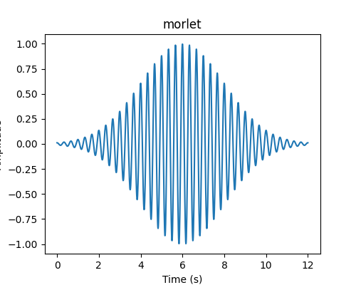
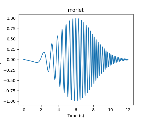
classmethod morlet(rate, frequency, width, samples=None, height=1, displacement=0, dfdt=0, filename='morlet')

Audio signal with the shape of the Morlet wavelet

Uses util.morlet_func() to compute the Morlet wavelet.

Args:

rate: float

Sampling rate in Hz

frequency: float

Frequency of the Morlet wavelet in Hz

width: float

Width of the Morlet wavelet in seconds (sigma of the Gaussian envelope)

samples: int

Length of the audio signal given as the number of samples (if no value is given, samples = 6 * width * rate)

height: float

Peak value of the audio signal

displacement: float

Peak position in seconds

dfdt: float

Rate of change in frequency as a function of time in Hz per second. If dfdt is non-zero, the frequency is computed as

f = frequency + (time - displacement) * dfdt

filename: str

Meta-data string (optional)

Returns:

Instance of Waveform

Audio signal sampling of the Morlet wavelet

Examples:

>>> from ketos.audio.waveform import Waveform
>>> # create a Morlet wavelet with frequency of 3 Hz and 1-sigma width of envelope set to 2.0 seconds
>>> wavelet1 = Waveform.morlet(rate=100., frequency=3., width=2.0)
>>> # show signal
>>> fig = wavelet1.plot()
>>> fig.savefig("ketos/tests/assets/tmp/morlet_standard.png")

>>> # create another wavelet, but with frequency increasing linearly with time
>>> wavelet2 = Waveform.morlet(rate=100., frequency=3., width=2.0, dfdt=0.3)
>>> # show signal
>>> fig = wavelet2.plot()
>>> fig.savefig("ketos/tests/assets/tmp/morlet_dfdt.png")
>>> plt.close(fig)

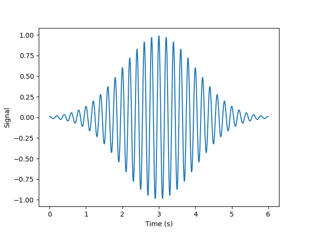
plot(show_annot=False, figsize=(5, 4), label_in_title=True, append_title='', show_envelope=False)

Plot the data with proper axes ranges and labels.

Optionally, also display annotations as boxes superimposed on the data.

Note: The resulting figure can be shown (fig.show()) or saved (fig.savefig(file_name))

Args:

show_annot: bool

Display annotations

figsize: tuple

Figure size

label_in_title: bool

Include label (if available) in figure title

append_title: str

Append this string to the title

show_envelope: bool

Display envelope on top of signal

Returns:

fig: matplotlib.figure.Figure

Figure object.

Example:

>>> from ketos.audio.waveform import Waveform
>>> # create a morlet wavelet
>>> a = Waveform.morlet(rate=100, frequency=5, width=1)
>>> # plot the wave form
>>> fig = a.plot()
>>> plt.close(fig)

resample(new_rate, resample_method='scipy')

Resample the acoustic signal with an arbitrary sampling rate.

TODO: If possible, remove librosa dependency

Args:

new_rate: int

New sampling rate in Hz

resample_method: str

Resampling method. Only relevant if rate is specified. Options are

• kaiser_best

• kaiser_fast

• scipy (default)

• polyphase

See https://librosa.github.io/librosa/generated/librosa.core.resample.html for details on the individual methods.

to_wav(path, auto_loudness=True)

Save audio signal to wave file

Args:

path: str

Path to output wave file

auto_loudness: bool

Automatically amplify the signal so that the maximum amplitude matches the full range of a 16-bit wav file (32760)